Replace legacy ETL (SAP R/3 & friends)

For: an enterprise data team that maintains a pile of ETL jobs (often hand-written, poorly documented) moving data out of SAP R/3 and other systems into a warehouse.

The problem. The existing ETL is fragile and opaque: scripts on a server, no clear dependency graph, painful to change, and it requires opening database access from the warehouse to production systems. You want something visual, governed, and without exposing SAP to the cloud.

What you'll build. An outbound-only connector that reads SAP read-only inside your network, a set of flows that extract and transform, and a pipeline that runs them in the right order on a schedule — with a monitoring view instead of log-tailing.

---

1. Install the on-prem connector

SAP shouldn't be reachable from the cloud — so AgentData reaches it instead. The connector runs inside your network, holds the DB credentials locally, and makes only outbound HTTPS calls. No inbound port, no firewall change.

In Sources → + Add source → On-premise, register a connector and download it for your OS:

• Pick ↓ macOS / ↓ Linux / ↓ Windows — a zip with the connector + installer for that OS.
• Set its .env: SOURCE_DATABASE_URL (a read-only SAP DB login) and STAGING_DATABASE_URL (a write/admin login for the staging DB). Download the pre-filled .env from the panel.
• Run the installer (bash install-linux.sh). Within ~30s the connector shows ● online with its version.

1234

Outbound HTTPS only — no inbound port, and never raw rows or credentials.

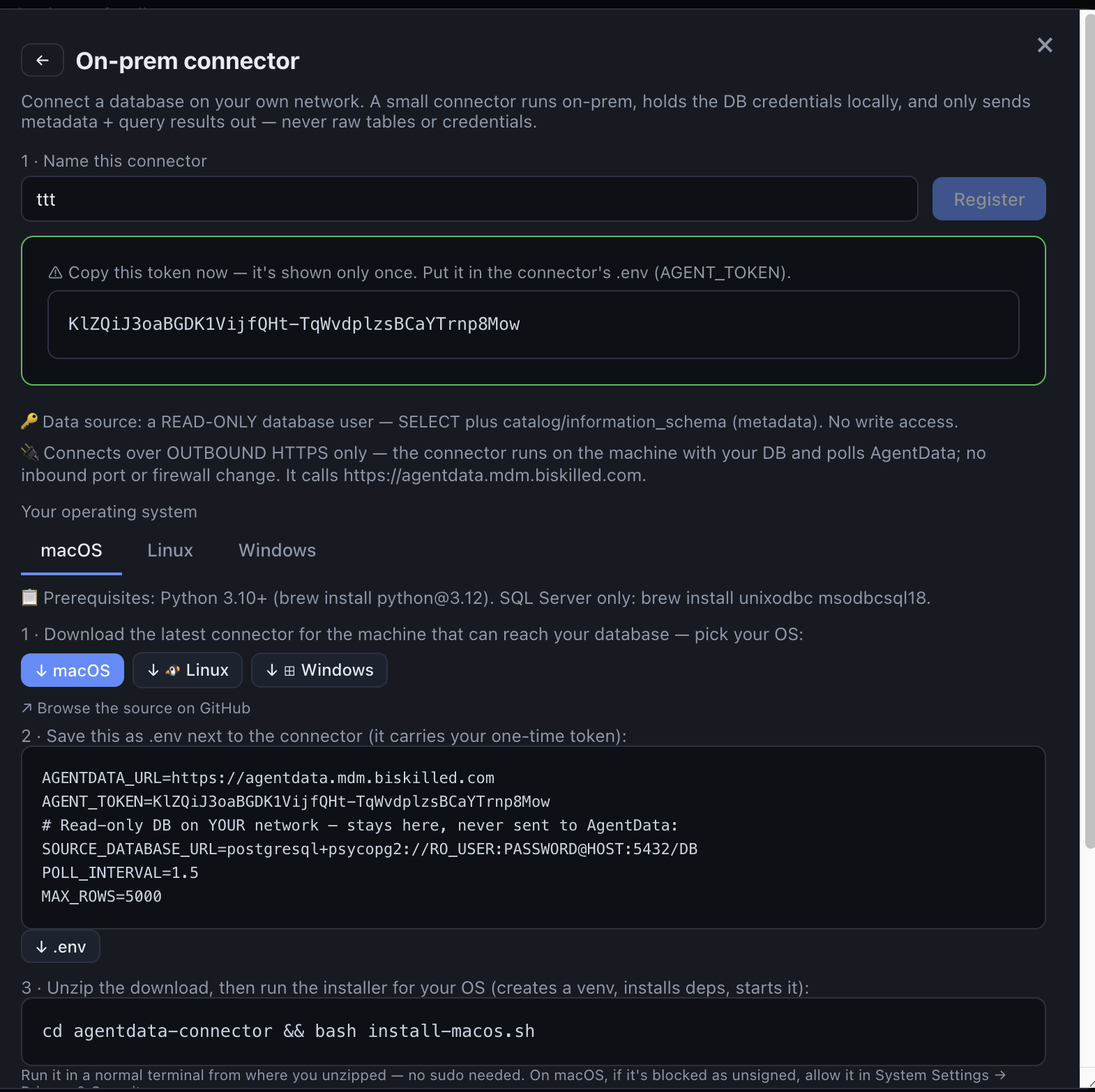
1. A one-time token — shown only once. It goes into the connector’s .env.
2. Download the latest connector for your OS — one click.
3. A pre-filled .env: backend URL, token, and your read-only + staging DB URLs. Download it.
4. Unzip, then run this command — no sudo. It comes online here in ~30s.

SAP's database

SAP R/3 stores its data in an underlying RDBMS (commonly Oracle or MS SQL Server). AgentData connects to that database read-only through the connector — the same way your reporting tools already do. Give it a least-privilege SELECT-only role.

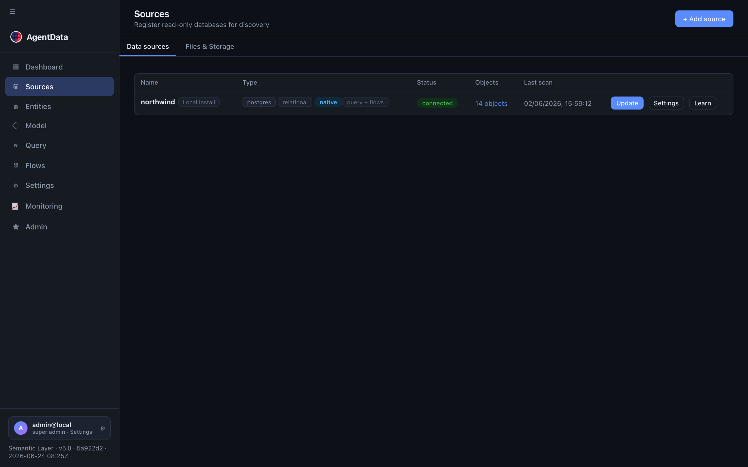
2. Register the source and a staging DB

• The connector you installed appears under On-premise; bind it as your SAP source (agent://…). AgentData profiles the tables read-only — rows never leave the network.
• Add a staging database (Flows → Staging) for control tables and load targets. It can be connector-backed too (writes happen on-prem), or a cloud Postgres/MySQL/SQL Server.

3. Build the extract + transform flows

Open Flows → + New flow. Each flow is one extract-transform-load unit. A typical SAP table → warehouse table flow:

1. Source — a table (e.g. KNA1 customers) or a SQL query for a join/filter you push down to SAP.

2. Transform — in the Designer, map source columns to clean target names, add calculated columns (expressions evaluated per engine), and rename/cast as needed. This replaces the transformation code in your old jobs.

3. Target — a new or existing table in staging, with a load type:

   • truncate_insert — full reload of a dimension,
   • upsert (on a key) — incremental updates,
   • delete_insert — partition reload.

   Set keys, create_if_missing, and recreate_on_change so schema drift is handled for you.

1234

This is where the logic from your old ETL scripts now lives — visible and editable.

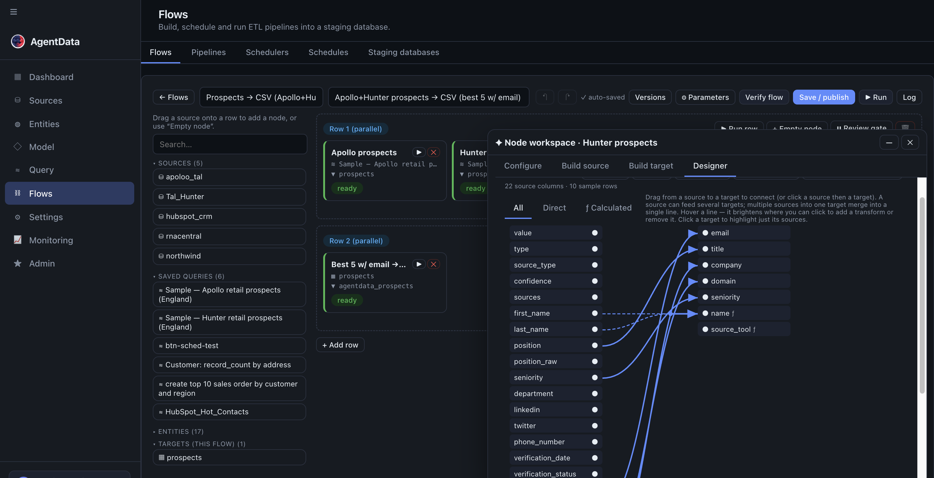
1. Pick a source: a table, or a push-down SQL query for a join/filter run on SAP.
2. Each flow is one extract→transform→load unit; build one per target table.
3. Designer: map and rename columns, add calculated columns, set the load type (truncate / upsert / delete-insert).
4. Save, then Run to check rows in / rows out.

Build one flow per target table — e.g. dim_customer, dim_material, fact_sales. Run each with ▶ Run and check rows in/out.

4. Orchestrate them as a pipeline (the DAG)

Dimensions must load before facts. Instead of encoding that order in cron offsets, model it visually.

Open Flows → Pipelines → + New pipeline:

• Drag your flows from the palette onto the canvas.
• Draw an arrow from each dimension flow to fact_sales (an arrow means "run this before that"). Flows with no remaining dependencies run in parallel; a flow whose upstream failed is skipped.
• Click ✨ Review to auto-arrange the graph into clean, evenly-spaced columns.
• Save pipeline.

1234

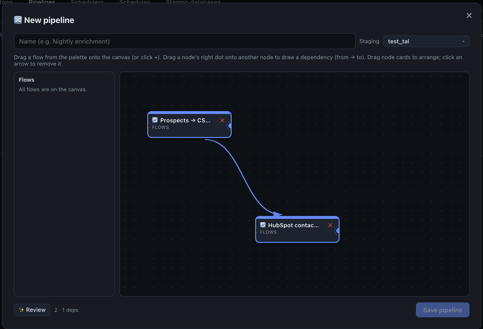
1. Drag a flow from the palette onto the canvas (or click +).
2. Drag a node’s right dot onto another node to draw a dependency — "run this before that".
3. Review: auto-arrange the graph into clean, evenly-spaced columns.
4. Save the pipeline — then run it via a scheduler or on demand.

5. Schedule and monitor

• Schedule: create a Scheduler (Flows → Schedulers), set Daily 02:00, and add your pipeline to it (a scheduler row can hold flows and whole pipelines). Or run the pipeline on demand with ▶ Run now.
• Monitor: the Monitoring view shows every run across flows and pipelines — status, rows, duration, errors — per tenant (super-admins see all tenants). No more SSH-ing to read logs.

123

A live log feed across every flow and pipeline run — no SSH-ing to read logs.

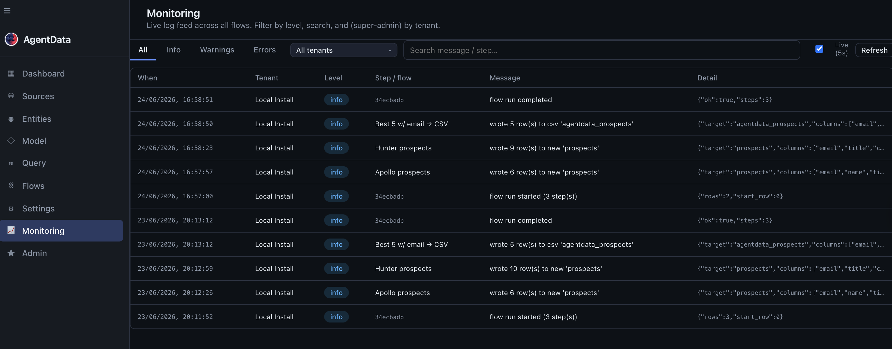
1. Filter by level (errors), by tenant, or search the message.
2. Each flow / pipeline step that ran.
3. What happened — rows written, run completed, or the error.

---

The result

The same nightly load your ETL did — now a readable DAG anyone on the team can inspect and change, scheduled in one place, monitored in one place, and with SAP reached read-only over an outbound-only connector so nothing is exposed to the cloud. Transformations live in the flow, not in tribal-knowledge scripts.

Next: point AgentData's discovery at the staging tables to get a governed semantic layer on top — so the data you just loaded is queryable in plain language.